How to draw a cycle time chart — Line up the motions in time and find where shortening pays off

Last updated: 2026-09-24 ／ Category: Mechanical and control design, cycle time

A cycle time chart lines up the motions of one cycle on a time axis and shows where shortening pays off. This guide is for mechanical and control designers who want to know at the quotation stage whether the required takt can be met.

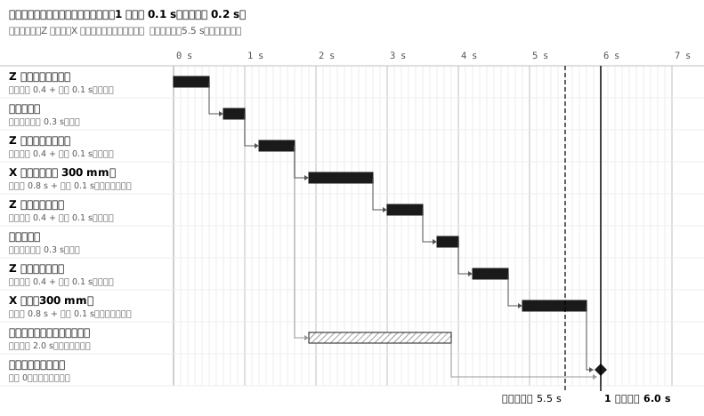
On a machine with a required takt of 5.5 s, one cycle of the transfer unit came to 6.0 s. The longest motion is the 2.0 s conveyor feed, yet a faster conveyor does not shorten the cycle. Which motion is worth shortening only becomes visible once the motions are lined up in time and the waits joined by arrows. This is a different diagram from the How to draw a timing chart of signal ON/OFF, and it is drawn on grid paper or in Excel.

One cycle of a transfer unit that picks the part at the conveyor's fixed position with Z and moves it to the jig with X. Each motion starts 0.2 s (the check interval) after the end of the motion it waits for. The note under each row gives the motion time and how completion is confirmed. Black: the longest path joined by waits, the one that sets the cycle. The hatched conveyor feed can be 1.9 s late without changing the cycle. On a phone, scroll the figure sideways or tap to open it.

1. Before drawing, settle what the takt means, the start and end points, and the row granularity

Is the required takt an upper limit for every cycle, or an average? The same chart passes or fails depending on which. On a palletizer, where the motion depends on the placing position, every cycle has a different length. Decide with the author of the specification which one is promised (the example uses the per-cycle upper limit).
The start and end of one cycle Write the start and end states on the chart. The cycle time at the acceptance test is measured between the same two points. The example runs from "Z up, X at pick side, part in position" until that state recurs.
One row per motion Cylinder advance and retract, chuck close and open, and each destination of an axis get a row of their own. Under each row, note the motion time and what confirms completion (the up-end sensor, in-position). The Z rise at the pick side and at the jig side wait for different things, so they are separate rows.

2. Estimate motion times as the catalogue value plus throttling and settling

Air cylinders — The bar length is the catalogue full-stroke time plus what the flow control adds. The catalogue time is measured under fast conditions: rated pressure, short tubing, needle fully open. Write it split in the note, "0.4 s + throttle 0.1 s", and redraw with measured values after commissioning.
Servo and electric axes — For a trapezoidal profile the time is distance L ÷ top speed v + t_a (the accel/decel time). 300 mm at 500 mm/s with t_a = 0.2 s takes 0.8 s, plus settling until in-position. If the distance is shorter than v × t_a the axis never reaches top speed, and the time is 2√(L × t_a ÷ v).
Robots — The catalogue standard cycle time is measured under the fastest conditions: a fixed payload and path, with coarse positioning that does not wait for the arm to settle. Get the time of each segment from the simulator with the part mass entered, and add the gripper open/close and the handover waits.
Check interval — The gap between the completion of one motion and the start of the next, often lumped as 0.2 to 0.5 s. Sensor response, PLC scan and output delay add up to a few tens of milliseconds. The rest is margin for variation and deliberate waits such as vacuum build-up, so cut whatever you cannot give a reason for.

3. Each start is "end of the awaited motion + check interval", joined by an arrow

Each motion starts at "end of the motion it waits for + check interval", and the wait arrow points there. When a motion waits for two others, draw two arrows and count from the later end. "Start of the next cycle" in the example waits for both the X return and the conveyor feed. With that row added, the cycle length can be read off as its start time.

If the next motion starts partway through a stroke, note the mid-stroke sensor under the row and draw the arrow from the middle of the bar. Whether that position is safe to start from is a question for mechanical design. The condition to move on is a sensor, not time. Advance on a timer alone and, when a part jams, the next motion starts before the previous one has finished.

4. The candidates for shortening are only on the longest path

The cycle length is set by the longest of the paths joined by wait arrows. In the example the path of the transfer unit's 8 motions (black) is 6.0 s. The conveyor feed ends at 3.9 s, so a faster one does not shorten the cycle. The candidates lie only on the black path.

Shorten the two X moves by 0.2 s each — Raise the top speed to 750 mm/s, 0.7 s with settling. The acceleration rises 1.5× too, so re-check the motor sizing. The cycle becomes 5.6 s, still 0.1 s short
Start the X return partway through the Z rise (jig side) — The X return starts at 4.6 s and the cycle becomes 5.7 s. Assume the chuck clears the jig 0.2 s into the rise and detect that with a mid-stroke sensor
Both together give 5.3 s, within the required takt

After shortening, redraw the chart and re-check the longest path. In the example the black path is unchanged at 5.3 s, but the conveyor's slack drops from 1.9 s to 1.2 s; if the feed exceeds 3.2 s, it becomes the longest path. When cylinder motions overlap, the air pressure drops and everything slows slightly, so check the supply as well.

5. Until the estimate is settled, draw it with Excel formulas

Draw in Excel until the estimate is settled; grid paper is for sketching additions by hand in a meeting. On paper, changing one motion time means redrawing everything after it. In Excel, draw no wait arrows: link the rows through the awaited motion in column B and the start formula, and paint the bars with conditional formatting. Drawn arrows do not follow when a motion time changes.

Lay out the table Columns A to D: motion, awaited motion (by name), motion time, check interval. Columns E to G: start, end, and the mark for the longest path; from column H rightwards, the scale in 0.1 s steps (column width 1 to 1.5). List the motions from row 3, and end with a zero-length "start of the next cycle" row (row 12 in the example).

Enter the scale and the start and end formulas Copy the formula in H1 to the right as far as BZ1 (7.0 s). Start and end use the formulas below: a row waiting for two motions uses MAX, and a row starting mid-stroke adds the seconds up to the sensor. ROUND is there because the rounding error of adding 0.1 shifts a bar by one column.

Cell	Formula	Meaning
H1	`=(COLUMN()-COLUMN($H$1))/10`	Scale (0, 0.1, 0.2…)
E3	0	Start of the first motion
F3	`=ROUND(E3+C3,1)`	End = start + motion time (copy down)
E4	`=ROUND(F3+D4,1)`	Start = end of the awaited motion + check interval
E11	`=ROUND(F5+D11,1)`	The conveyor feed waits for Z up (pick side)
E12	`=ROUND(MAX(F10,F11)+D12,1)`	Start of the next cycle. Waits for two. This value is the cycle length
E10	`=ROUND(E9+0.2+D10,1)`	When the X return starts partway through Z up (jig side), at 0.2 s

Paint the bars and the required takt with conditional formatting Select H3:BZ12 and create the three conditional-formatting rules below. The required takt goes in C14 under the table; change the value and the border moves with it. If no colour appears, check "Applies to" in Manage Rules, and for printing check the gridlines (Making a timing chart in Excel).

Rule	Formula
Dark fill (longest path)	`=AND(H$1>=$E3,H$1<$F3,$G3="●")`
Light fill	`=AND(H$1>=$E3,H$1<$F3,$G3<>"●")`
Left border at the required takt (5.5 in C14)	`=H$1=ROUND($C$14,1)`

Trace the longest path Trace backwards from the start-of-next-cycle row and put ● in column G of each row on the path. Follow the motion that set the start (the one MAX picked); those bars turn dark and the candidates stand out. Painting a bar cell by hand changes nothing, because the conditional format sits on top.

6. Where people trip: hidden margins, the first cycle, waits between units

Padding motion times without saying why — Write margins in the row note together with the reason. Mixed in, they hide both where to shorten and how the measured values differ. When the takt is not met, keep the margins that have a reason and revisit speeds, equipment and overlaps instead
Drawing only the steady-state cycle and not the first one — Draw the first cycle on a separate chart. Right after start there is no previous part to wait for, and moves from the home position are added. Customers care about the seconds from start to the first part out, so specify it separately from the acceptance cycle
Assuming each unit gets the whole takt — Draw wait arrows across units. Otherwise the time spent waiting for another unit to retreat stays invisible, and the chart exceeds the takt once joined up. The same applies when the units are designed separately

7. The takt and the start and end points on the chart become the acceptance conditions

Write on the chart the required takt, whether it is a per-cycle limit or an average, and the start and end states. The acceptance test measures several consecutive cycles with parts flowing and no waiting for upstream or downstream machines. The first cycle on a winter morning tends to be slow because the grease is stiff. If a per-cycle limit is promised, decide beforehand whether that one counts.

The rows and wait arrows of the chart are the steps and the move-on conditions of the operation How to draw a PLC control flowchart. Signal handovers with other machines and robots are drawn as signal order in the Timing Chart Editor.

yk.builds